Head Related Transfer Functions (HRTFs)

A large body of research has been carried out on HRTF measurement (see Hebrank and Wright, 1974, Mehrgardt and Mellert, 1977, Butler and Belendiuk, 1977, Shaw and Teranishi, 1968, Shaw, 1974, Shaw, 1975, Shaw and Vaillancourt, 1985, Gardner and Martin, 1994, 1995, Møller et al, 1995, Hammershøi and Møller, 1996, Carlile and Pralong, 1994, Pralong and Carlile, 1994 and Blauert, 1997).

The external ear transfer functions are measured in the above publications at various places along the ear canal, which gives rise to different responses. However, since up to 12-14 kHz only the longitudinal mode is present in the ear canal, the variation of the position of the microphone does not distort the directionally dependent HRTFs.

The initial assumption made during this work was that the highest resolution possible is required for the mesh models of the head and pinnae. It was not clear at that stage what accuracy is required and how sensitive will be the modelling of the acoustical response to geometry approximations. There are currently a few techniques available to obtain a computer model by scanning a physical model. These include: Computed Tomography (CT), Magnetic Resonance Imaging (MRI), 3-D ultrasonic imaging, etc. These are generally used for internal scanning for medical purposes. The main advantage of the 3-D laser scanner technique used in this research is that it can produce fairly quickly an accurate mesh of the surface made out of triangles

In the initial work, the Cyberware 'Head and Face' colour 3-D scanner had been used. This scanner includes the 3030/RGB digitising head and the PS motion system. It is mainly used for medical applications, anthropometry, human interface, and in the film industry. The geometry is captured by means of an optical range-finding system that produces around a half of a million interconnected triangles and their vertices in approximately 15 seconds. We refer to this scanner as having a 'low-resolution'.

To begin with, it was found in the scanning stage, that the accuracy of the pinna, which is our most important part of the head, was poor, since during the motion of the scanner the laser beam detects only unhidden parts. In the initial trials using the KEMAR head, the rear part of the pinnae were significantly distorted, and more importantly, the resulting concha was much shallower then the original rubber ear of KEMAR, and without the details of the cavum and cymba concha, helix, antihelix and fossa of helix. However, only after a set of simulations, it was found that another scanning technique was required for high accuracy modelling of the pinna.

Although still based on the technology of laser scanning, the Cyberware 'Mini model' 3-D scanner is based on the high-resolution 3030RGB/HIREZ scan head with a mid-size high-resolution motion system. It moves slowly from side to side in the horizontal plane in a straight line, parallel to the object. The principle of operation is similar to the 'head and face' scanner, but with software controlled, the data is accumulated through repeated scans at different angles of the pinna. In this way, almost every curvature can be captured correctly. Even the ear canal geometry can be obtained, by providing an additional model with the original's cross-section. Then, the software matches the 'internal' data with its own 'external' data by matching overlapping sections. The duration of this scanning procedure is much longer, of the order of a few hours; before any post-processing is applied to fix connectivity, rough surface, holes, etc.

A few tools were developed and used to integrate the two scans into a single mesh model for both KEMAR head and YK head. Two types of decimated KEMAR models are presented below. In both cases the original data included more than 400000 triangles (around 200000 vertices). The target was to obtain a suitable BEM mesh that could be used to modelling at the maximum frequency possible with the IBEM in-core solver . The mesh on the right was decimated using our proposed algorithm that produces homogeneously distributed vertices, thus optimising its size, geometry, and maximum frequency. This resulted in approximately 23000 elements that can be used up to 15 kHz if four elements per wavelength are assumed (for the ipsilateral ear), and 10 kHz if six elements per wavelength are assumed (for the contralateral ear).

When a conventional mesh decimation algorithm was used (the mesh in the middle, optimised for computer graphics applications), and the number of elements was limited to 23000 elements, a mesh with non-uniform distribution of vertices was obtained, where planar areas were described with less triangles, and complex areas retained a higher density of triangles to preserve the geometry. Note that with both decimation algorithms the rendered image (on the left) is very similar. This mesh in the middle could be investigated using the BEM reliably only up to 1 kHz (!). This emphasises the significance of optimising the mesh distribution while retaining the accuracy of complex shapes such as the pinna.

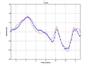
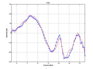
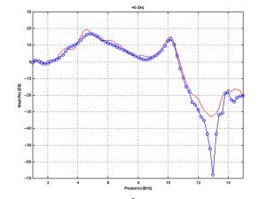
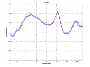
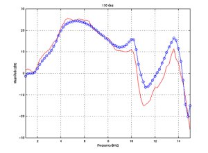
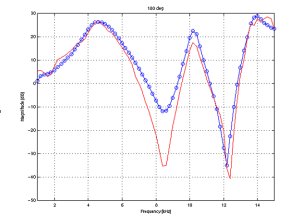
BEM simulation and measurement comparison

The following figures demonstrate the accuracy of the simulation results when compared to measurements at various angles in the horizontal plane.

The same simulated and measured responses are shown at discrete angles. These show that errors of <1 dB appear up to 15 kHz. At other angles where sharper notches are found errors increase locally at the position of the notch. It should be noted that median plane simulation and measurement do not impose great difficulty from the SNR point of view, since there are no effects of the shadowing due to the head, which have strong attenuation at high frequencies.